Аннотация

Introduction. Deep learning is a modern technique for image processing and data analysis with promising results and great potential. Successfully applied in various fields, it has recently entered the field of agriculture to address such agricultural problems as disease identification, fruit/plant classification, fruit counting, pest identification, and weed detection. The latter was the subject of our work. Weeds are harmful plants that grow in crops, competing for things like sunlight and water and causing crop yield losses. Traditional data processing techniques have several limitations and consume a lot of time. Therefore, we aimed to take inventory of deep learning networks used in agriculture and conduct experiments to reveal the most efficient ones for weed control.
Study objects and methods. We used new advanced algorithms based on deep learning to process data in real time with high precision and efficiency. These algorithms were trained on a dataset containing real images of weeds taken from Moroccan fields.
Results and discussion. The analysis of deep learning methods and algorithms trained to detect weeds showed that the Convolutional Neural Network is the most widely used in agriculture and the most efficient in weed detection compared to others, such as the Recurrent Neural Network.
Conclusion. Since the Convolutional Neural Network demonstrated excellent accuracy in weed detection, we adopted it in building a smart system for detecting weeds and spraying them in place.

Ключевые слова

Digital agriculture, weed detection, machine learning, deep learning, Convolutional Neural Network (CNN), Recurrent Neural Network (RNN)

ВВЕДЕНИЕ

In our growing digital world, machine learning is at the core of data science [1]. Machine learning techniques and computing power play an essential role in the analysis of collected data. They have focused on representing input data and generalizing learned predictive models to future data [2]. Data representation has a dramatic effect on machine learner performance. Proper data representation can lead to high performance even with straightforward machine learning. In contrast, poor representation of data with advanced complex machine learning can lead to decreased performance [3].

Deep learning is an important branch of machine learning that has emerged to achieve impressive results in the field of artificial intelligence. Its strength is in its ability to automatically create powerful data representation through layers of learning without human intervention, thus ensuring great precision of analysis [4]. In comparison with shallow learning algorithms, deep learning uses supervised and unsupervised techniques and machine-learning approaches to automatically learn the hierarchical representation of multi-level data for feature classification [5, 6]. This deep learning composition is inspired by the representation of human brain for processing natural signals. It has attracted the academic community lately due to its performance in different research fields, such as agriculture.

More recently, a number of technologies common in industry have been applied to agriculture, such as remote sensing, the Internet of Things (IoT), and robotic platforms, leading to the concept of “smart agriculture” [7, 8]. Smart agriculture is important to face agricultural production challenges in terms of productivity, environmental impact, and food security. To tackle these challenges, it is necessary to analyze agricultural ecosystems, which involves constant monitoring of different variables. These operations create data that can be used as input values and processed with varying analysis techniques in deep learning to identify weeds, diseases, etc.

The objects of our study were two neural networks, namely the Convolutional Neural Network (CNN) and the Recurrent Neural Network (RNN). A CNN is an artificial neural network used for image recognition and processing [9]. It is specially intended for handling pixel information. A CNN is viewed as a powerful artificial intelligence (AI) image processing system that employs deep learning to perform generative and descriptive tasks. It commonly uses machine vision, which includes image and video recognition, as well as recommendation systems and natural language processing (NPL) [10]. A RNN, in its turn, is an artificial neural network essentially utilized in discourse identification and programmed regular language treatment. RNNs are intended to perceive successive attributes and information utilization patterns needed to foresee likely scenarios [11]. Therefore, the use of a RNN in image classification requires optimization with the long shortterm memory (LSTM) technique to reduce the risk of gradient vanishing [12]. In this study, we compared these two techniques of deep learning with other state of the art techniques in order to create an optimized model and train it to detect weeds. We aimed to create an intelligent system that could detect weeds and spray them locally to avoid wasting herbicides and protect the environment.

ОБЪЕКТЫ И МЕТОДЫ ИССЛЕДОВАНИЯ

In this study, we used various methods, devices, techniques, and libraries to study deep learning in crop planting and train the deep learning models on a database that includes images for relevant and smart weed detection. The following sections contain complete descriptions of these methods.

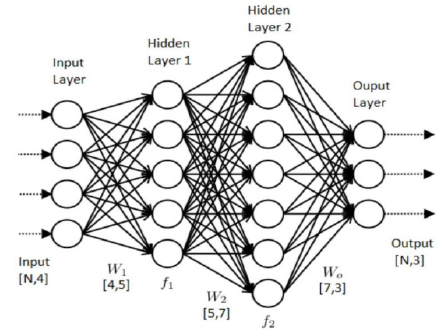
Deep learning. This method came to expand machine learning (ML) and added a lot of complexity and depth to the model based on artificial neural networks (ANNs). A neural network is a system designed to resemble the neural organization of the human brain. A more complex definition would be that a neural network is a computational model made up of artificial neurons connected to each other and resulting in a network architecture. This architecture has specific parameters called weights. Adjusting them, we can enhance the accuracy of our model. This type of networks contains many layers, each with a specific mission. Their number determines the complexity of the network. We can find three layers in a small neural network: the input layer, the hidden layer, and the output layer. Each of these layers is comprised of hubs called “nodes” and has a given assignment, as the name suggests. The input layer is liable for recovering information and giving it to the following layer. The hidden layer plays out all the back-end assignments of the calculation and change of information utilizing different capacities that permit its portrayal in a progressive manner through a few degrees of abstraction [13]. There can be multiple layers hidden in a neural network as needed. Several parameters influence the laying of various layers, and the goal is always to obtain a high degree of accuracy. The output layer passes the consequence of the hidden layer, as shown in Fig. 1.

Deep learning has various applications ranging from natural language to image processing. Its important advantage is the learning of functionalities, or automatic extraction of functionalities from raw data. Functionalities of more significant levels of a progressive system are framed by the arrangement of lower level functionalities.

Deep learning can tackle more perplexing issues well and rapidly by utilizing more complex layers, which permits enormous parallelization. These complex algorithms increase classification accuracy and reduce errors, provided there are large, well-prepared and sufficient data sets to describe the problem and the layers are well constructed.

The profoundly progressive construction and great learning capacity of deep learning algorithms permit them to perform classification and expectation with high accuracy. They are versatile and adaptable to a wide range of exceptionally complex problems. Deep learning has numerous applications in data management (e.g. video, images), tending to be applied to any type of information, like natural language, speech, and continuous or point data [15].

The main drawbacks of deep learning could be long learning time and a need for powerful hardware suitable for parallel programming (Graphics Processing Unit, Field-programmable Gate Array), while conventional strategies like Scale Invariant Feature Transform (SIFT) or Support Vector Machine (SVM) have less difficult learning measures [16]. In any case, the testing time is quicker in deep learning tools and most of them are more accurate. The subsections below present the most common deep learning techniques.

Convolutional Neural Network (CNN). In deep learning, convolutional neural networks (CNNs) are a class of profound feedforward ANNs that has been effectively applied to computer vision. In contrast to an ANN, whose tediously prepared prerequisites may be unfeasible in some huge scope issues, a CNN can learn complex issues quite rapidly because of weight sharing and more complex layers utilized.Convolutional neural networks can increase their likelihood of correct classifications, provided there are sufficiently large data sets (i.e. hundreds to thousands of measurements, depending on the complexity of the problem under investigation) available to describe the problem. They are made up of different convolutional layers, grouped and/or fully connected. Convolutional layers perform operations to extract distinct features from the input images whose dimensionality is reduced by grouping the layers together, while fully connected layers perform classification operations. They usually exploit the learned high-level functionalities at the last layer in order to classify the input images into predefined classes. Many organizations have successfully applied this technique in various fields, such as agriculture where it accounts for 80% of all methods used [17]. An example of CNN architecture is shown in Fig. 2 [18].

Figure 2 shows different representations of the training dataset created by applying various convolutions to certain layers of the network. Training always begins as the most general at the level of the first layers, which are larger, and becomes more specific at the level of the deeper layers.

A combination of convolutional layers and dense layers makes the production of good precision results possible. There are various “successful” architectures that researchers commonly use to start building their models instead of starting from scratch. These include AlexNet, the Visual Geometry Group (VGG) (shown in Fig. 2), GoogleNet, and Inception-ResNet, which uses what we call “transfer learning.” Besides, there are various tools and platforms that allow researchers to experience deep learning. The most popular are TensorFlow, Theano, Keras (an application programming interface on top of TensorFlow and Theano), PyTorch, Caffe, TFLearn, Pylearn2, and Matlab. Some of these tools (e.g. Caffe, Theano) integrate popular platforms such as those mentioned above (e.g. AlexNet, VGG, GoogleNet) in the form of libraries or classes [19].

Recurrent Neural Network (RNN). Recurrent neural networks (RNNs) are another type of neural networks that is used to solve difficult machine learning problems involving sequences of inputs. Some RNN architectures for sequence prediction issues are:
1. One-to-Many: sequence yield, for picture captioning;
2. Many-to-One: sequence in input contribution, for sentiment investigation; and
3. Many-to-Many: sequence for synchronized input, machine translation and output sequences, typically processing operations for video classification.

RNNs have connections with loops, adding feedback and memory to networks over time. This memory has come to replace traditional learning that relies on individual patterns. It allows this type of network to learn and generalize through a sequence of inputs. When an out is produced, it is copied and sent back to the recurrent network [20]. To make a decision, it considers the current entry and the exit it learned from the previous entry. An example of RNN architecture is shown in Fig. 3.

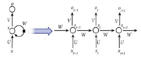
Figure 3 shows an RNN for the entire sequence. For example, if a sentence consists of five words, the network will unwind into a neural network of five layers, one layer for each word. The formulas that govern calculations in an RNN are as follows:
– x_t entered at time t.
– U; V; W are the parameters that the network will learn from the training data.
– St is the hidden state at time t. It is the “memory” of the network. St is calculated based on the previous hidden state and the entry to the current step:

where f is a nonlinear function such as ReLu or Hyperbolic tangent (TanH).

Ot (2) is the exit at time t. A well-known example here is the prediction of a word in the sentence. When we want to know the next word in the sentence, it will show a vector of possibilities in the vocabulary.

Deep learning applications in agriculture. Applications of deep learning in agriculture are spread across several areas, the most popular being weed identification, land cover classification, plant recognition, fruit counting, and crop type classification. According to Fig. 4, which shows deep learning models in crop planting, CNNs and RNNs account for 80% and only 5% of all methods, respectively.

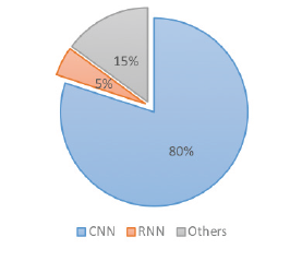
The low ratio of RNNs in agriculture is due to the fact that traditional RNNs have unstable behavior with the vanishing gradient and therefore are not used in image classification. For this reason, we will discuss an advanced RNN in this article that uses the LSTM technique for image classification in weed identification. Weeds are plants that grow spontaneously on agricultural soils where they are unwanted. The growth of these plants causes competition with crops for space, light, and water. Herbicides are the first tool used to fight against weeds, but they present secondary risks for man and nature. Therefore, we need to think about ways to reduce their effects. In this study, we proposed an intelligent system that automatically detects weeds and contributes to localized spraying of infected areas only. To identify weeds, we processed photos of crops and classified them to apply specific herbicides.

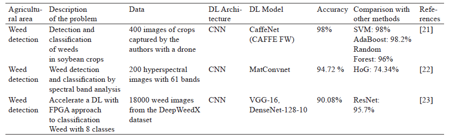
Weeds can be classified according to the size of their leaves into grass categories (dicot and monocot). This division is adequate since grasses and broadleaf weeds are differentiated in treatment due to the selectivity of some herbicides to the specific group. Herbicide application works best if treatment is targeted at the specific class of weed. Several studies have shown the success of CNNs in comparison with RNNs and other deep learning techniques used for weed identification [21–23].

Technical details. From a technical standpoint, almost all of the research has used popular CNN architectures such as AlexNet, VGG, and Inception- ResNet, or combined CNNs with other procedures. All the experiments that exploited a well-known system also used a deep learning framework, with Caffe being the most famous. Noteworthily, most studies that only had small datasets to train their CNN models exploited the power of data augmentation to artificially increase the number of training images to enhance their accuracy. They used translations, transposition, and reflections, as well as modified the intensities of the RGB Channels, and that is what we did to prepare our dataset.

Also, the majority of related works included image preprocessing steps, where each image in the dataset was scaled down to a smaller size before being used as input into the model, such as 256×256, 128×128, 96×96, 60×60 pixels, or converted to CNN grayscale architectures to take advantage of transfer learning. Transfer learning exploits already existing knowledge of certain related tasks in order to increase the efficiency of learning the problem at hand, refining pre-trained models when it is impossible to train the network on the data from the beginning due to a small set of training data or the resolution of a complex problem. We can get significant results if we rely on weights from other models that were previously trained on big datasets [24]. In our case, these are preformed CNNs that have already been trained on datasets related to different class numbers. The authors of related work mainly used large datasets to train their CNN models, in some cases containing thousands of images. Some of them came from well-known and publicly available sources such as PlantVillage, MalayaKew, LifeCLEF, and UC Merced. In contrast, some authors produced their own datasets for their research needs, as we can see in Table 1. The table also shows whether the authors compared their CNN-based approach with other techniques used to solve the problem under study, as well as the precision of each model. Therefore, conventional precision of the model’s response must be exactly the expected response.

Application of an optimized RNN in weed detection. All the studies referred to above have used CNN architectures to create deep learning models that detect weeds. Also, they have compared them with other models in terms of accuracy and error. RNNs, however, do not feature much in these works, which means they are hardly used in this field of agriculture, especially for image classification. That is why we aimed to create an optimized RNN model with the long short-term memory (LSTM) technique as an alternative to the traditional RNN [25]. We trained this RNN-LSTM model on our dataset in order to compare the results with those obtained by the CNN above. First, we loaded the dataset that was already used in a previous experiment. This database contained a set of weeds known in our region and spread over four classes. Then, we built an RNN model and trained it on the database created using the following parameters: inputs = 28, step = 28, neuron = 150, output = 10, epoch = 20, Softmax function. LSTMs were introduced in our model in order to improve the RNN standards. The RNN model we created is shown in Fig. 5.

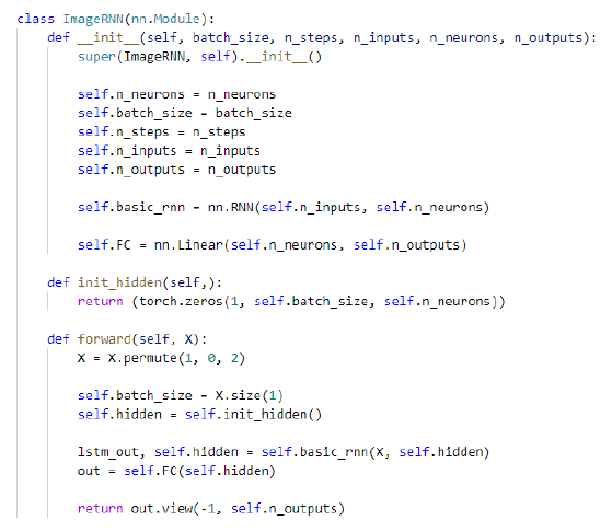
To design this deep learning model, we used the python code, as shown in Fig. 6.

The above code includes the initialization function _ _init_ _, which defines some variables. The fully connected layer follows the basic RNN by “self.FC” that allows data to flow through the RNN layer and then through the fully connected layer, also using the function “init_hidden” that exploits hidden weights with zero values.

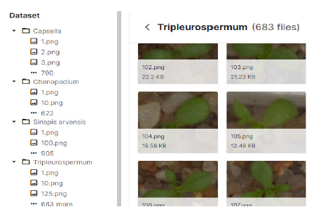
The database used to train the proposed RNN and CNN models comprised about 3000 images taken in a wheat field with a digital camera (Sony 6000) under different lighting conditions (from morning to afternoon in sunny and cloudy weather). We combined these images with those from the online Kaggle repository dataset. The images featured four types of weeds that propagate in our region. They corresponded to four classes to be identified by our model (Fig. 7). A well-prepared database is a very important factor in deep learning. We applied preprocessing and dataaugmentation techniques on the same data to generate other learning examples through different manipulations (flip, orientation, contrast, crop, exposure, noise, brightness…). These techniques reduced the model’s performance.

РЕЗУЛЬТАТЫ И ИХ ОБСУЖДЕНИЕ

Before training the model, we added all necessary functions (Fig. 8). Firstly, we specified the device runtime to use during training, determined in the python code by torch.device(...). This function gives commands to the program to use the GPU (Graphics Processing Unit) if it is available. Otherwise the CPU (Central Processing Unit) will be used as a default device. The GPU acts as a specialized microprocessor. It is swift and efficient for matrix multiplication and convolution. Parallelism is often cited as an explanation. The GPU is optimized for bandwidth, while the CPU is optimized for latency. Therefore, the CPU has less latency, but its capacity is lower than that of the GPU. In other words, CPUs are not suited to handle massive amounts of data, while GPUs can provide large amounts of memory. The CPU is responsible for performing all kinds of calculations, whereas the GPU only handles graphics calculations. Since our dataset was not large, we used an i7 CPU with 2.80GHz and 8G of RAM.

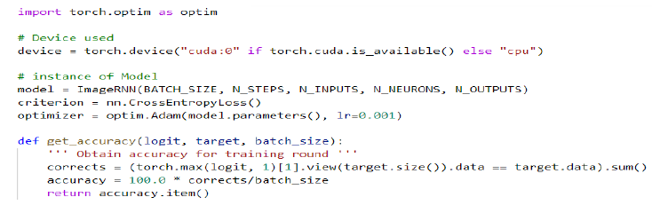
Then, we create an instance of the model with the ImageRNN(...) function, with its own configuration and parameters, the criterion represents the function we will use to get the loss of the designed model. To do this process, it is sufficient to use the function: nn.CrossEntropyLoss(), which is a softmax function utilized as boundaries log probabilities and followed by a negative log-likelihood loss activity over the output of the model. The code shows how to provide this to the criterion.

We add an optimization function that recalculates the weights based on the current loss and updates it. This is done using the Optim.adam function, which requires setting the model parameters and learning rate. To display the results and get the accuracy, we will use the get_accuracy(...) function, which computes the accuracy of the model given the log probabilities and target values for each epoch. All these functions are shown in the figure below.

After training the model on 20 epochs, we obtained relevant results (Figs. 9 and 10).

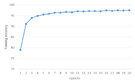
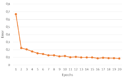
There are different ways and measures to evaluate the performance of a classification model. The performance measures often used are precision, kappa, recall, and others [26]. We were therefore interested in the model’s accuracy and error rate. Accuracy is a proportion of genuine expectations in relation to the absolute number of input pictures. The error rate measures the difference between the model’s predictions and the real images in the training set [27]. Figures 9 and 10 show the accuracy and error for each epoch. In particular, Fig. 10 shows how the neural network gradually decreased the error to arrive at 0.9. According to Fig. 9, the training accuracy reached 97.58% due to a set of factors, such as the dataset, optimization function, and the adjustment of weights and biases.

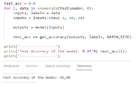
Figure 11 shows how the model performed on the test images. The display of predictions on test images is a technique to test the final solution in order to confirm the real predictive power of the network. We computed the accuracy on our dataset to test how well the model performed on the test images. Figure 11 shows a value of 96.40%, which means that the predictions on the test images were well classified.

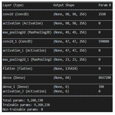
These results indicated a good performance of the LSTM-RNN on our dataset. According to the three figures above, this model updates with every step, adjusting weights to reduce error and increasing accuracy using a backpropagation algorithm and gradient descent. In addition to the studies that were based on CNNs, we also built a CNN-based model (Fig. 12) and trained it on the same dataset that we used in the RNN experiment.

Our results were close to those reported by the authors referred to above.

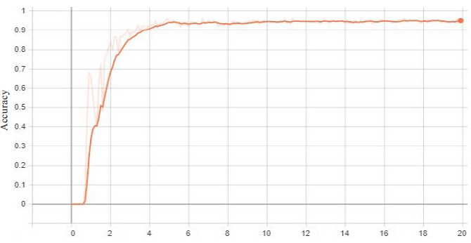
The training was run on our local machine and after a few times it reached 98% validation accuracy. The model showed good results after 9 h of training. Figure 13 shows accuracy taken from Tensboard.

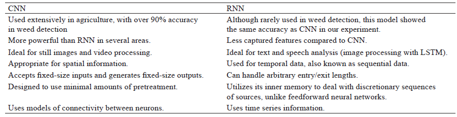
To sum up, CNNs are preferred for interpreting visual data, sparse data or data that does not come in sequence. Recurrent neural networks, however, are designed to recognize sequential or temporal data. They make better predictions by considering the order or sequence of data concerning previous or next data nodes. Applications where CNNs are particularly useful include face detection, medical analysis, drug discovery, and image analysis. RNNs are useful for linguistic translation, entity extraction, conversational intelligence, sentiment analysis, and speech analysis. Our experiment also showed that RNNs can be used to classify images if we add the LSTM technique. Based on literature and our results, we compared the characteristics of RNNs and CNNs and summarized them in Table 2.

Our experimentation clearly shows why CNNs are so widely used in agriculture despite the abundance of other deep learning techniques. In addition, we proved that a RNN can also be used to detect weeds, but with less efficiency and more effort. Therefore, we recommend the CNN as the best suited deep learning technique for more efficient weed detection as the basis for smarter precision farming.

ВЫВОДЫ

Precision agriculture encompasses several areas of application, such as plant and leaf disease detection, land cover classification, plant recognition, and weed identification to name the most common uses. The development of precision agriculture requires new monitoring, control, and information technologies, including deep learning. This paper presents an overview and a comparative study of deep learning tools in crop planting. First, we looked at agriculture to describe its current problems, specifically weed detection. Then, we listed the technical characteristics of popular deep learning techniques. After that, we created a CNN and a RNN and trained them on our dataset to compare their overall accuracy. The results showed that the optimized RNN model (RNN with LSTM) can also be used to classify images with acceptable accuracy. Hence, a RNN combined with the LSTM is suitable for detecting weeds among other techniques, but a CNN always comes first in terms of speed and accuracy. In future work, we intend to use other metrics to compare the results, such as recall and Kappa. We will also try to develop a platform combining the RNN with the CNN to achieve the best accuracy. These results will be used to build an intelligent system based on Raspberry Pi 4 that can detect weeds in real time and spray them in their area.

КОНФЛИКТ ИНТЕРЕСОВ

The authors declare no conflict of interest regarding the publication of this article.

БЛАГОДАРНОСТИ

This research is part of the Digital Agriculture doctorate project that involves a group of doctors from the Limati Laboratory at Sultan Moulay Slimane University in Morocco.

СПИСОК ЛИТЕРАТУРЫ

1. Ferguson AL. Machine learning and data science in soft materials engineering. Journal of Physics Condensed Matter. 2018;30(4). https://doi.org/10.1088/1361-648X/aa98bd.
2. Momennejad I. Learning structures: Predictive representations, replay, and generalization. Current Opinion in Behavioral Sciences. 2020;32:155–166. https://doi.org/10.1016/j.cobeha.2020.02.017.
3. Peng S, Sun S, Yao Y. A survey of modulation classification using deep learning: Signal representation and data preprocessing. IEEE Transactions on Neural Networks and Learning Systems. 2021. https://doi.org/10.1109/TNNLS.2021.3085433.
4. Salloum SA, Alshurideh M, Elnagar A, Shaalan K. Machine learning and deep learning techniques for cybersecurity: A review. Advances in Intelligent Systems and Computing. 2020;1153:50–57. https://doi.org/10.1007/978-3-030-44289-7_5.
5. Alloghani M, Al-Jumeily D, Mustafina J, Hussain A, Aljaaf AJ. A systematic review on supervised and unsupervised machine learning algorithms for data science. In: Berry MW, Mohamed A, Yap BW, editors. Supervised and unsupervised learning for data science. Cham: Springer; 2020. pp. 3–21. https://doi.org/10.1007/978-3-030-22475-2_1.
6. Nowicki RK, Grzanek K, Hayashi Y. Rough support vector machine for classification with interval and incomplete data. Journal of Artificial Intelligence and Soft Computing Research. 2020;10(1):47–56. https://doi.org/10.2478/jaiscr-2020-0004.
7. Jabir B, Falih N, Sarih A, Tannouche A. A strategic analytics using convolutional neural networks for weed identification in sugar beet fields. Agris On-line Papers in Economics and Informatics. 2021;13(1):49–57. https://doi.org/10.7160/aol.2021.130104.
8. Jabir B, Falih N. Digital agriculture in Morocco, opportunities and challenges. 2020 IEEE 6th International Conference on Optimization and Applications (ICOA); 2020; Beni Mellal. Beni Mellal: Sultan Moulay Slimane University; 2020. https://doi.org/10.1109/ICOA49421.2020.9094450.
9. Duda P, Jaworski M, Cader A, Wang L. On training deep neural networks using a streaming approach. Journal of Artificial Intelligence and Soft Computing Research. 2020;10(1):15–26. https://doi.org/10.2478/jaiscr-2020-0002.
10. Zhang C, Lin Y, Zhu L, Liu A, Zhang Z, Huang F. CNN-VWII: An efficient approach for large-scale video retrieval by image queries. Pattern Recognition Letters. 2019;123:82–88. https://doi.org/10.1016/j.patrec.2019.03.015.
11. Lin JC-W, Shao Y, Djenouri Y, Yun U. ASRNN: A recurrent neural network with an attention model for sequence labeling. Knowledge-Based Systems. 2021;212. https://doi.org/10.1016/j.knosys.2020.106548.
12. Shen J, Ren Y, Wan J, Lan Y. Hard disk drive failure prediction for mobile edge computing based on an LSTM recurrent neural network. Mobile Information Systems. 2021;2021. https://doi.org/10.1155/2021/8878364.
13. LeCun Y, Bengio Y, Hinton G. Deep learning. Nature. 2015;521(7553):436–444. https://doi.org/10.1038/nature14539.
14. Araujo VJS, Guimaraes AJ, Souza PVD, Rezende TS, Araujo VS. Using resistin, glucose, age and BMI and pruning fuzzy neural network for the construction of expert systems in the prediction of breast cancer. Machine Learning and Knowledge Extraction. 2019;1(1):466–482. https://doi.org/10.3390/make1010028.
15. Kulkarni A, Halgekar P, Deshpande GR, Rao A, Dinni A. Dynamic sign language translating system using deep learning and natural language processing. Turkish Journal of Computer and Mathematics Education. 2021;12(10):129–137.
16. Huu PN, Ngoc TP, Manh HT. Proposing gesture recognition algorithm using HOG and SVM for smart-home applications. In: Vo N-S, Hoang V-P, Vien Q-T, editors. Industrial networks and intelligent systems. Cham: Springer; 2021. pp. 315–323. https://doi.org/10.1007/978-3-030-77424-0_26.
17. Kamilaris A, Prenafeta-Boldú FX. A review of the use of convolutional neural networks in agriculture. Journal of Agricultural Science. 2018;156(3):312–322. https://doi.org/10.1017/S0021859618000436.
18. Nash W, Drummond T, Birbilis N. A review of deep learning in the study of materials degradation. npj Mater Degrad. 2018;2(1). https://doi.org/10.1038/s41529-018-0058-x.
19. Bousetouane F, Morris B. Off-the-shelf CNN features for fine-grained classification of vessels in a maritime environment. In: Bebis G, Boyle R, Parvin B, Koracin D, Pavlidis I, Feris R, et al., editors. Advances in visual computing. Cham: Springer; 2015. pp. 379–388. https://doi.org/10.1007/978-3-319-27863-6_35.
20. Ganai AF, Khursheed F. Predicting next word using RNN and LSTM cells: Stastical language modeling. 2019 Fifth International Conference on Image Information Processing (ICIIP); 2019; Shimla. Solan: Jaypee University of Information Technology; 2019. p. 469–474. https://doi.org/10.1109/ICIIP47207.2019.8985885.
21. dos Santos Ferreira A, Freitas DM, da Silva GG, Pistori H, Folhes MT. Weed detection in soybean crops using ConvNets. Computers and Electronics in Agriculture. 2017;143:314–324. https://doi.org/10.1016/j.compag.2017.10.027.
22. Farooq A, Hu J, Jia X. Analysis of spectral bands and spatial resolutions for weed classification via deep convolutional neural network. IEEE Geoscience and Remote Sensing Letters. 2018;16(2):183–187. https://doi.org/10.1109/LGRS.2018.2869879.
23. Lammie C, Olsen A, Carrick T, Azghadi MR. Low-power and high-speed deep FPGA inference engines for weed classification at the edge. IEEE Access. 2019;7:51171–51184. https://doi.org/10.1109/ACCESS.2019.2911709.
24. Harsono IW, Liawatimena S, Cenggoro TW. Lung nodule detection and classification from Thorax CT-scan using RetinaNet with transfer learning. Journal of King Saud University – Computer and Information Sciences. 2020. https://doi.org/10.1016/j.jksuci.2020.03.013.
25. Sherstinsky A. Fundamentals of recurrent neural network (RNN) and long short-term memory (LSTM) network. Physica D: Nonlinear Phenomena. 2020;404. https://doi.org/10.1016/j.physd.2019.132306.
26. Gupta S, Agrawal A, Gopalakrishnan K, Narayanan P. Deep learning with limited numerical precision. Proceedings of the 32 nd International Conference on Machine; 2015; Lille. Lille: JMLR W&CP; 2015. p. 1737–1746.
27. Pak M, Kim S. A review of deep learning in image recognition. 2017 4th International Conference on Computer Applications and Information Processing Technology. Kuta Bali; 2017. p. 367–369. https://doi.org/10.1109/CAIPT.2017.8320684.