Аннотация

The dynamic models of elements of technological systems with perfect mixing and plug-flow hydrodynamics are based on the systems of algebraic and differential equations that describe a change in the basic technological parameters. The main difficulty in using such models in MathWorks Simulink™ computer simulation systems is the representation of ordinary differential equations (ODE) and partial differential equations (PDE) that describe the dynamics of a process as a MathWorks Simulink™ block set. The study was aimed at developing an approach to the synthesis of matrix dynamic models of elements of technological systems with perfect mixing and plug-flow hydrodynamics that allows for transition from PDE to an ODE system on the basis of matrix representation of discretization of coordinate derivatives. A sugar syrup cooler was chosen as an object of modeling. The mathematical model of the cooler is formalized by a set of perfect reactors. The simulation results showed that the mathematical model adequately describes the main regularities of the process, the deviation of the calculated data from the regulations did not exceed 10%. The proposed approach significantly simplifies the study and modernization of the current and the development of new technological equipment, as well as the synthesis of algorithms for controlling the processes therein.

Ключевые слова

Mathematical modeling, dynamic systems, sugar syrup cooler, MathWorks Simulink™

ВВЕДЕНИЕ

The main way to study the regularities of technological heat and mass exchange processes in the food industry is to make a full-scale experiment. In many cases, it results in a number of insurmountable difficulties due to its cost, the ability of engineering implementation of the control parameters, etc. Due to this, the development of adequate and correct mathematical models of technological processes that allow us to replace a full- scale experiment is a relevant task.

The processes of heat and mass transfer in moving media can be simulated on the basis of the Navier- Stokes equation, but the equations obtained are not always suitable for analysis. Therefore, the perfect models of a flow pattern have become widespread in practice:   perfect mixing models (they describe a change in concentration, temperature, etc. in compounders), plug-flow models (they describe a change in concentration, temperature, etc. in the case of a plug-flow going through an apparatus), cellular models and others [1–3]. The mathematical models of such apparatus are called perfect mixing reactors (PMR), plug-flow reactors (PFR), etc.

A Simulink interactive graphical simulation environment is widely used for the computer modeling of technological processes that allows using block diagrams in the form of directed graphs to construct dynamic models, including discrete (continuous and hybrid), non- linear models and models with singularities. In addition, the Simulink environment includes the tools for building, modeling and studying control systems which allows for the simulation of a process and control system within a single integrated environment [4].

When modeling perfect reactors, the conversion of the equations to describe a technological process into a set of blocks of the visual programming environment of Simulink is necessary. In the case of systems of ordinary differential equations (ODE), an input signal integration unit and a MathWorks™ numerical methods library are used, as well as the method for representing ODE or an ODE system in the form of a structural Simulink model [5, 6]. In the case of partial differential equations that describe, for example, plug-flows, the heat conductivity equation, etc., there is a problem of bringing PDE to an ODE equation or system. One of the approaches used in the transition from PDE to ODE is the use of integral transformations, for example, Fourier transformations and Laplace transformations [7, 8], and the disposal of spatial derivatives. It is not always possible to obtain a solution to such equations in analytical form. In addition, the implementation of direct and inverse integral transformations by means of Simulink for an arbitrary input signal is difficult. The other approach is to use numerical methods for solving PDE (finite elements, finite differences, etc.) and to integrate program blocks into the structural model of Simulink using the custom functions implemented on the basis of such programming languages as MathWorks and universal ones like C ++ [9]. In this case, it is possible to implement the entire arsenal of available tools for the numerical solution of PDE, but any modification of an object model entails the need for changing the function code and debugging it, thereby violating the objectoriented principle of Simulink – the separation of the internal structure and interface of a model. One of the approaches is based on the discretization of only the spatial variable using the finite difference method, while the derivatives with respect to time remain continuous and PDE is represented as the Cauchy problem for the ODE system [10]. The implementation of each equation of the ODE system results in the formation of rather cumbersome structural models in Simulink, and the compact representation of such systems in a matrix form is relevant [11, 12]. In this case, it is necessary to replace the expansion of spatial derivatives with matrix equations [12]. [13] shows such a representation of a one-dimensional heat conductivity equation for Simulink.

 Thus, the relevant task is to develop a method for representing typical perfect reactors using matrix ordinary differential equations (MODE) and to implement structural models therewith in Simulink.

ОБЪЕКТЫ И МЕТОДЫ ИССЛЕДОВАНИЯ

To synthesize the matrix dynamic model of a typical perfect reactor, it is necessary to perform the following sequence of actions:
 – to select the model of a perfect reactor suitable for describing the structure of the flow in process equipment (this issue is considered in detail in the special literature, for example, in [1–3]);
– to draw up the corresponding differential equation. As a result, for each perfect reactor, one or more ODE or PDE are obtained with the corresponding initial and boundary conditions;
– to solve the resulting equation or a set thereof with respect to the highest derivative with respect to time;
– to discretize spatial derivatives (in the case of their presence) in accordance with the accepted form of finite-difference approximation;
– to replace each PDE by a set of ODE using the replacement of partial derivatives with respect to the spatial variable by the corresponding matrix equation. For example, the first derivative of the temperatureis replaced as follows:

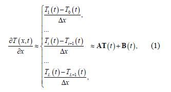
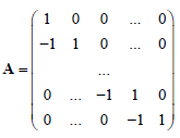
where is the decomposition matrix of the first derivative, and 

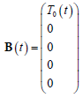
is a vector to define the boundary condition. The second derivative can be defined as 

 

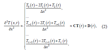
where 

is the decomposition matrix of the second derivative, and 

is a vector to define the boundary conditions.

–   then, in accordance with the procedure described in [5], to draw up a structural diagram of a perfect reactor model in the form of Simulink blocks that solve MODE taking into account the fact that the signals transmitted from block to block are vectors and matrices and the corresponding multiplication operations will be performed according to the rules of matrix multiplication. In this case, the time derivatives will be integrated using numerical methods from the Simulink library;

–      to define the parameters of the model that characterize flow hydrodynamics, the geometry of perfect reactor models and the thermophysical properties of process media;

–   to create input and output streams to build process equipment models in the form of a system of perfect reactors and additional subsystems, if necessary; and

– to design a reactor model in the form of a subsystem in the Simulink format.

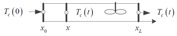
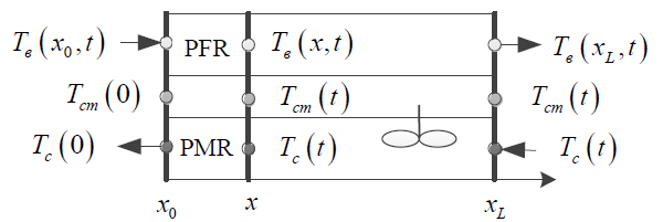
Let us consider the synthesis process of a dynamic matrix mathematical model using a sugar syrup cooler as an example which is used for fondant sweet processing lines [14]. The cooler is a cylindrical body 1, inside which a rotating screw 2 (рассмотрите pushes sugar syrup forward (Fig. 1). The body 1 is equipped with a cooling jacket made in the form of a closed spiral canal (CSC) 3 cooling water (a coolant) is fed through. As a result of the heat exchange between the syrup and the coolant through the wall of CSC that separates them, the temperature of the syrup decreases, which results in the crystallization of sucrose from the fondant syrup and the formation of fondant mass.

The quality indicators of the finished product (fondant mass) are the size of sucrose crystals and their proportion in the total volume of fondant mass. In turn, the disperse composition of fondant mass depends entirely on both the cooling parameters of fondant syrup–temperature, the intensity of removal of heat from the syrup–and its thermophysical and rheological properties that change during the crystallization sucrose process [14]. 

To model the heat exchange between the syrup and the coolant, let us select the models of perfect reactors. In view of the intensive mixing of sugar syrup with a rotating screw, the complexity of the mathematical description resulting from the mixing of the three- dimensional temperature pattern, as well as the necessity of conjugation of the geometric coordinates of cooling water and sugar syrup flows, let us estimate in the first approximation the average temperature of sugar syrup according to the length of the cylindrical body 1. Averaging the sugar syrup temperature according to the length of the body by integrating the PMR equation with respect to the variable x and dividing it by the length of the body, we obtain an equation that corresponds to PFR in structure. For the cooling water flow, let us neglect the temperature distribution over the cross-sectional area of the canal and choose a PMR model. The perfect reactors are physically separated by a wall through which there is a heat exchange between the coolant and sugar syrup. Let us neglect the thermal effects as a result of the process of crystallization of sucrose from the syrup, as well as heat exchange with the environment. Let us assume that the wall temperature is constant along the length.

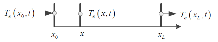
Let us consider the synthesis of the PFR model in accordance with the diagram in Fig. 2.

If the structure of the syrup flow corresponds to the PFR model, an equation of a temperature change taking heat transfer into account can be used for the mathematical description of this flow [2]. It will be an ordinary differential equation with respect to the temperature of the syrup TC

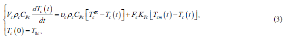
where Vc is the volume of the perfect mixing area, m3 ; Pс is density of sugar syrup,  is the specific heat capacity of sugar syrup,  is the volumetric flow rate,  is the flow temperature at the inlet to the perfect mixing area; Fc is the surface of heat exchange between the syrup and the wall of CSC,   is the coefficient of heat transfer from the syrup to the center of the wall of CSC,   is the temperature of the center of the wall of CSC, °C.

To solve the equation in Simulink, let us use the technique described in [5] and represent Eq. 3 in the form of Simulink blocks (Fig. 3) having previously solved Eq. 3 with respect to the derivative.

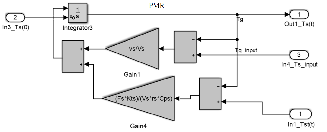
Let us consider the synthesis of the model of a plug-flow reactor (Fig. 4).

If the structure of the flow corresponds to the plug- flow model (the model is based on the assumption that the temperature is constant in the cross section and there is no longitudinal mixing), then for the mathematical description of this flow, an equation taking heat transfer into account can be used [1]

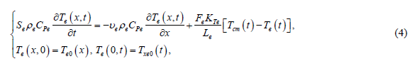
where 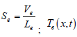 is the function of spatial and time distribution of temperature of the coolant flow; Vв is the volume of the plug-flow area, m3 ; Pв is the density of the coolant, kg/m3 ; Сpв is the specific heat capacity of the coolant,  is the volumetric flow rate, is the flow temperature at the inlet to the plug-flow area; Fв is the surface of heat exchange between the coolant and the wall of CSC, m2 ; KTв is the coefficient of heat transfer from the coolant to the center of the wall of CSC, W/(m2 × K). Let us bring Eq. 4 to a finite-difference form and solve it with respect to the derivative 

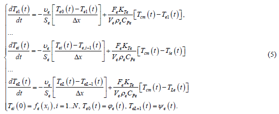
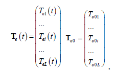
Let us define the vector of the current temperature at the points of coordinate partitioning and the initial conditions 

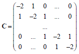
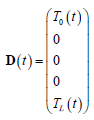
Let us represent the first derivative in the form of a matrix expression [4] 

where) is the decomposition matrix of the first derivative, 

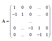
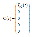
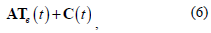
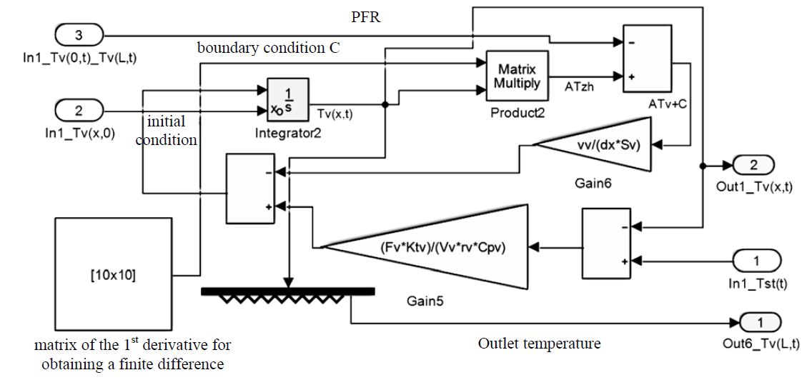
is a vector to define the boundary condition. Then let us write the ODE system (5) as a matrix ODE 

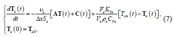
and represent it in the form of a structural Simulink model (Fig. 5). Since the statement of the problem implies that the heat capacity of the wall that separates the heat carrier flows cannot be neglected, then these equations will be supplemented by an equation of a change in the temperature of the wall that separates the media Tсm(t) 

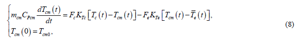
where  is the wall mass, kg; is the specific heat capacity of the wall,  is the average temperature of the coolant over the entire length calculated as

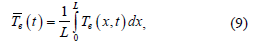
and when partitioning it by N elements with respect to x it is replaced with the sum

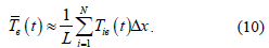
Let us represent it in the form of a structural Simulink model (Fig. 6).  

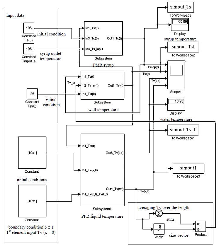
As a result, a set of subsystems for modeling perfect reactors is formed. To compile a cooler model, it is only necessary to connect the subsystems into a single design scheme in accordance with Fig. 7 and set the model parameters. In this case, the mathematical model of the cooler can be described by a system of scalar and matrix ODE 

 

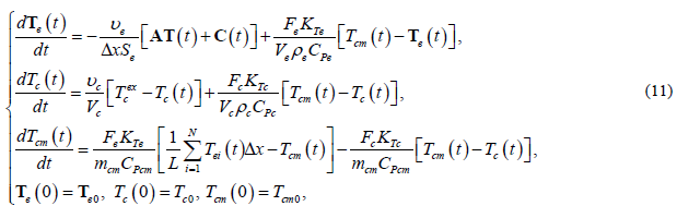
with the parameters [14, 15]: the heat capacity of the coolant  ; the heat capacity of the wall  ; the heat capacity of the syrup  ; the heat exchange area of the  coolant-wall  ; the heat exchange area syrup wall ; the wall mass mст = 25.465 kg; the cross-sectional area inside   ; the coefficient of thermal conductivity of the wall   the density of the wall material (copper)  ; the density of the coolant  ; the density of syrup the coefficient of heat transfer from the coolant to the  wall   ; the coefficient of heat transfer from the syrup to the wall  ; the coefficient of heat transfer from the syrup to the center of the wall  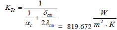 ; the coefficient of heat from the coolant to the center of the wall  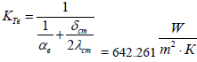 ; the discretization interval Δ x = 2.07 m; the number of discretization elements along the length N = 10; the thickness of the wall of CSC, ; the length of CSCL = 20.7 m; the volumetric flow rate of the coolant ; the syrup volumetric flow rate  ; the initial temperature of the coolant  the initial temperature of syrup  the initial wall temperature ; the volume of the area of PFR ; and the syrup volume in PMR 

The structural model in the form of Simulink blocks is shown in Fig. 8, the simulation results are shown in Figs. 9–11. The studies and computer experiment were carried out at the Voronezh State University of Engineering Technology. 

РЕЗУЛЬТАТЫ И ИХ ОБСУЖДЕНИЕ

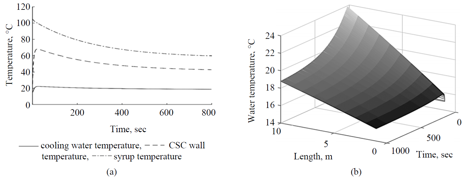
The data in Fig. 9 show that the sugar syrup is cooled from the initial temperature of 105°С to 60°С within 600–800 sec, which is consistent with the technological regulations for fondant mass production. The further cooling of syrup does not result in a decrease in the temperature of the finished product. The deviation of the calculated data from the regulations did not exceed 10%.

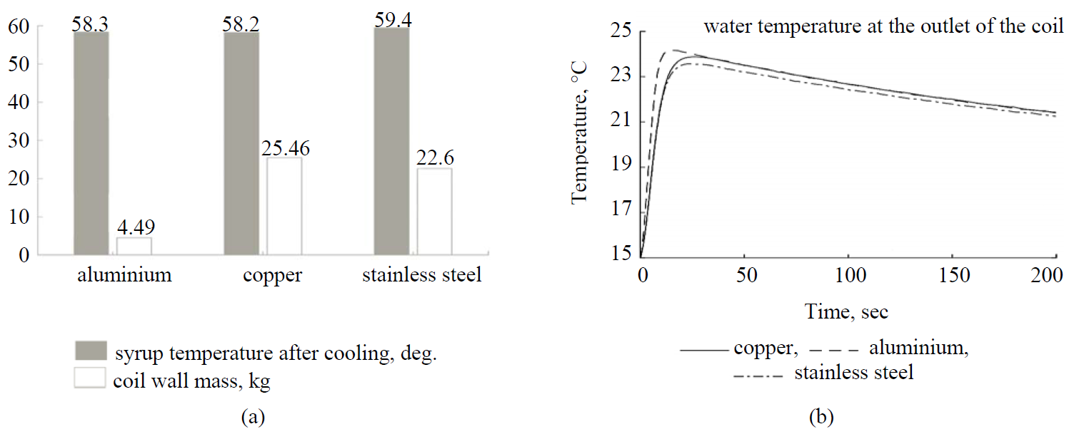
The model developed with the help of this approach makes it possible to obtain the estimates of temperatures at the outlet from the cooler in real time (Fig. 9a) which makes it possible to study the dynamics of the technological process and synthesize a control system. It is also possible to estimate the temperature distribution in terms of both the time and length of the heat exchange surface of CSC (Fig. 9b). In addition, by varying the parameters of a mathematical model, it is possible to estimate their effect on the technical and economic indicators of a process, for example, when changing the material which CSC is made of (Fig. 10a), and also to predict a change in the dynamic characteristics of a process (Fig. 10b). 

When the syrup is cooled, its viscosity significantly changes which entails a change in the hydrodynamics of the syrup flow and conditions of heat exchange between the coolant and syrup through the wall that separates them. The introduction of a temperature correction in the calculation of syrup viscosity makes it possible to take into account a change in the coefficient of thermal conductivity from the syrup to the wall of CSC. For example, using the data of [16], let us approximate the dependence of syrup viscosity on temperature using the Arrhenius equation 

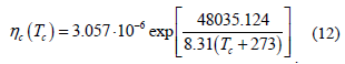
Then, taking into account the dependence of syrup viscosity on temperature, it is possible to estimate the coefficients of heat transfer and thermal conductivity from the syrup to the wall of CSC for each temperature and to clarify the syrup cooling dynamics (Fig. 11). In this case, the heat transfer and thermal conductivity coefficients are calculated with the help of an additional Matlab Function block from the Simulink library that performs the continuous calculation of the heat transfer and thermal conductivity coefficients according to the current values of syrup temperature delivered to the block input. 

The further refinement of the cooler model can be due to, first, taking into account the thermal effects resulting from the crystallization of sucrose from the syrup and, secondly, taking into account the design features of a typical fondant beater (feeding cooling water into the shaft of the conveying screw, separating the machine body and cooling water jacket into three sections in each of which the heat is removed from the syrup with various intensity). 

ВЫВОДЫ

The presented approach makes it possible to implement the mathematical models of perfect reactors in Simulink by discretizing the spatial variable and to pass over to matrix ordinary differential equations, which makes it possible to convert them into Simulink blocks. The approach is also applicable to other models of perfect reactors, which makes it possible to build the libraries of typical perfect reactors of Simulink for the synthesis of heat and mass transfer equipment that makes it easy to integrate them into a single system of synthesis, study, and debugging of Simulink control systems. Within the framework of Simulink simulation systems, a further refinement of the obtained simplest models based on perfect reactors by introducing variable model parameters, nonlinearities, control circuits, etc. is possible. This significantly simplifies the study and modernization of the current technological equipment and the development of new equipment, as well as the synthesis of control algorithms for the processes therein. 

КОНФЛИКТ ИНТЕРЕСОВ

The authors declare no conflict of interest. 

БЛАГОДАРНОСТИ

The authors would like to thank Professor Yu.Yu. Gromov of the Tambov State Technical University for all his help and support. 

ФИНАНСИРОВАНИЕ

The study was conducted with the support of the Applied Mathematics and Mechanics Department, the Voronezh State Technical University.  

СПИСОК ЛИТЕРАТУРЫ

1. Berk Z. Food Process Engineering and Technology: Second Edition. New York: Academic Press, 2013. 720 p.
2. Van Boekel M. Kinetic Modeling Reactions in Foods. Florida : CRC Press, 2009. 767 p.
3. Harriot P. Chemical Reactor Design. New York: Marcel Dekker, 2003. 99 p.
4. MathWorks. Available at: http://matlab.ru/. (accessed 02 October 2017).
5. Herman R. Solving Differential Equations Using SIMULINK. Published by R.L. Herman, 2016. 87 p.
6. Gray M.A. Introduction to the Simulation of Dynamics Using Simulink. Boca Raton, Florida : CRC Press 2011. 308 p.
7. Duffy D.G. Transform Methods for Solving Partial Differential Equations, Second Edition. Boca Raton, Florida : CRC Press, 2004. 728 p.
8. Wong M.W. Partial differential equations: topics in fourier analysis. Boca Raton; London; New York: CRC Press, 2013. 184 p.
9. Ozana S. and Pies M. Using Simulink S-Functions with Finite Difference Method Applied for Heat Exchangers. Proceedings of the 13th WSEAS International Conference on SYSTEMS. Greece, Rodos, 2009, p. 210–215.
10. Mazzia A. and Mazzia F. High-order transverse schemes for the numerical solution of PDEs. Journal of Computational and Applied Mathematics, 1997, vol. 82, no. 1–2, pp. 299–311. DOI: https://doi.org/10.1016/S0377-0427(97)00090-3.
11. LeVeque R.J. Finite Difference Methods For Ordinary and Partial Differential Equations. Philadelphia: SIAM, 2007. 339 p.
12. Moler C.B. Numerical Computing with MATLAB. Philadelphia: SIAM, 2004. 336 p.
13. Hunt A.B.R., Lipsman R.L., Rosenberg J.M., et al. A Guide to MATLAB: for Beginners and Experienced Users. Cambridge: Cambridge University Press, 2006. 302 p.
14. Dragilev A.I., Khromeenkov V.M., and Chernov M.E. Tekhnologicheskoe oborudovanie: khlebopekarnoe, makaronnoe i konditerskoe [Technological equipment: bakery, macaroni and confectionery]. St. Petersburg: Lan Publ., 2016. 430 p. (In Russ.).
15. Dragilev A.I. and Rub M.D. Sbornik zadach po raschetu tekhnologicheskogo oborudovaniya konditerskogo proizvodstva [Problem book on confectionery technological equipment calculation]. Moscow: DeLi Print Publ., 2005. 244 p. (In Russ.).
16. Salov V.S. and Nazarenko S.V. Temperatura kipeniya i vyazkost' sakharnykh rastvorov [Boiling point and viscosity of sugar solutions]. News institutes of higher Education. Food technology, 1999, nos 2–3, pp. 69–71. (In Russ.).